---
title: "In Search of Intuition: Transforms"
description: "From guitar tuners to discrete event simulators"
author: "Adam Fillion"
date: "2026-01-23"
categories: [probability, statistics, simulation]
draft: false
format:
html:
code-fold: true
---
As an electrical engineering undergrad, a minor project I completed was an automatic guitar tuner. An inductive sensor detects the guitar string movement, we convert this to a digital signal, analyze it, manipulate the string tensions with some motors we found in a box somewhere, and hopefully end up with an accurately tuned guitar.
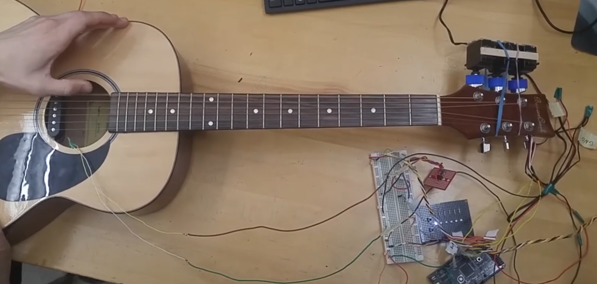
Steve Jobs probably wouldn't have been fond of our industrial design, but this was a scrappy prototype.
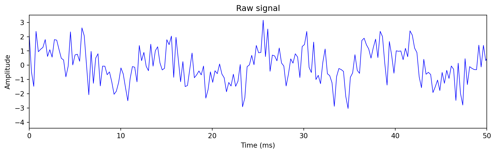
At the core of this project is digital signal analysis — converting a time series signal to the frequency domain so that we can easily identify the dominant frequency and make adjustments.
The raw signal looked something like this:
```{python}
#| code-fold: false
import numpy as np
import matplotlib.pyplot as plt

sample_rate = 4000
duration = 0.1
t = np.linspace(0, duration, int(sample_rate * duration))

fundamental = 82.41  # E2 string
signal = (np.sin(2*np.pi*fundamental*t) +
          0.5*np.sin(2*np.pi*2*fundamental*t) +
          0.3*np.sin(2*np.pi*3*fundamental*t) +
          1*np.random.randn(len(t)))

plt.figure(figsize=(12, 3))
plt.plot(t*1000, signal, 'b-', linewidth=0.8)
plt.xlabel('Time (ms)')
plt.ylabel('Amplitude')
plt.title('Raw signal')
plt.xlim(0, 50)
plt.show()
```
Although it's easy for humans to visually spot the dominant frequency with a fuzzy peak to peak analysis, it's much more difficult to do so programmatically within the time domain. All the software sees is a stream of numbers representing an amplitude - and devising algorithms for this peak analysis can quickly become unwieldy due to noise, or multiple simultaneous string pluckings. I challenge you to write an algorithm for this that can run on an low power Arduino circuit board.
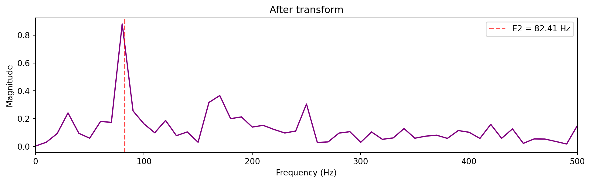
So instead of struggling with time series data points, we filter the signal with a bandpass filter, then apply a Fourier transform [[2]](#references) to "transform" the X-axis from time to frequency.
```{python}
#| code-fold: false
from scipy.fft import fft, fftfreq
from scipy.signal import butter, lfilter

# Butterworth bandpass filter for environmental noise
low, high = 10, 500
nyq = sample_rate / 2
b, a = butter(4, [low/nyq, high/nyq], btype='band')
filtered_signal = lfilter(b, a, signal)

N = len(t)
frequencies = fftfreq(N, 1/sample_rate)[:N//2]
spectrum = np.abs(fft(filtered_signal))[:N//2] * 2/N

plt.figure(figsize=(12, 3))
plt.plot(frequencies, spectrum, 'purple', linewidth=1.5)
plt.xlabel('Frequency (Hz)')
plt.ylabel('Magnitude')
plt.title('After transform')
plt.xlim(0, 500)
plt.axvline(x=82.41, color='red', linestyle='--', alpha=0.7, label='E2 = 82.41 Hz')
plt.legend()
plt.show()
```
The spike at ~82 Hz is our E string. Harmonics are the smaller spikes [[5]](#references). From here, the tuning algorithm is trivial.
This is indistinguishable from magic (if you're a Renaissance era academic).
## Years Later....
Since my undergrad, I haven't used transforms much - it turns out they don't come up much in distributed systems. Fortunately, I recently needed them to build a component of a discrete event simulator I am working on.
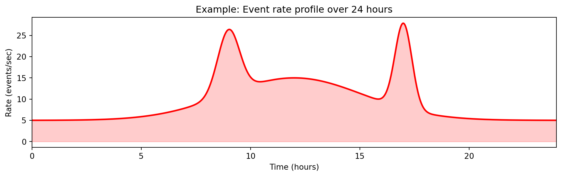
When running simulations, you may want to manipulate the simulation using a time based profile - for example to change a variable as a function of time or, in my case, generate events at a certain rate [[3]](#references).
```{python}
#| code-fold: true
import numpy as np
import matplotlib.pyplot as plt

t = np.linspace(0, 24, 1000)  # 24 hour period

def rate(t):
    # Base rate with morning ramp, evening cooldown
    base = 5 + 10 * np.exp(-((t - 12)**2) / 20)  # Peak at noon
    # Traffic spikes
    spike1 = 15 * np.exp(-((t - 9)**2) / 0.5)   # 9am spike
    spike2 = 20 * np.exp(-((t - 17)**2) / 0.3)  # 5pm spike
    return base + spike1 + spike2

plt.figure(figsize=(12, 3))
plt.plot(t, rate(t), 'r-', linewidth=2)
plt.fill_between(t, 0, rate(t), alpha=0.2, color='red')
plt.xlabel('Time (hours)')
plt.ylabel('Rate (events/sec)')
plt.title('Example: Event rate profile over 24 hours')
plt.xlim(0, 24)
plt.show()
```
One thing you need to know about many simulations is that they are event-based, every event has a timestamp, and this defines the ordering of the simulation, but nothing "happens" in between events - the event itself is what moves the simulation time forward.
The simulation core is a time ordered heap, where events are pushed and popped from the heap as the simulation progresses and comes to life.
```{ojs}
//| echo: false
viewof simStep = Scrubber(d3.range(0, 15), {
  autoplay: true,
  loop: true,
  delay: 800,
  label: "Simulation step"
})
```
```{ojs}
//| echo: false
{
  const width = 600, height = 200;
  const svg = d3.create("svg").attr("viewBox", [0, 0, width, height]).attr("width", "100%");

  // Events with timestamps
  const allEvents = [
    {t: 0.5, label: "A"}, {t: 1.2, label: "B"}, {t: 2.1, label: "C"},
    {t: 3.0, label: "D"}, {t: 3.8, label: "E"}, {t: 4.5, label: "F"},
    {t: 5.2, label: "G"}, {t: 6.1, label: "H"}, {t: 7.0, label: "I"},
    {t: 8.2, label: "J"}, {t: 9.1, label: "K"}, {t: 10.0, label: "L"},
    {t: 11.5, label: "M"}, {t: 12.3, label: "N"}, {t: 13.0, label: "O"}
  ];

  const processed = allEvents.slice(0, simStep);
  const heap = allEvents.slice(simStep, Math.min(simStep + 5, allEvents.length));
  const currentTime = simStep > 0 ? allEvents[simStep - 1].t : 0;

  // Timeline
  const xScale = d3.scaleLinear().domain([0, 14]).range([50, width - 20]);
  svg.append("line").attr("x1", 50).attr("y1", 50).attr("x2", width - 20).attr("y2", 50)
    .attr("stroke", "#ccc").attr("stroke-width", 2);
  svg.append("text").attr("x", width/2).attr("y", 20).attr("text-anchor", "middle")
    .attr("font-size", "12px").text(`Simulation time: ${currentTime.toFixed(1)}`);

  // Current time marker
  svg.append("line").attr("x1", xScale(currentTime)).attr("y1", 35).attr("x2", xScale(currentTime)).attr("y2", 65)
    .attr("stroke", "#e74c3c").attr("stroke-width", 3);

  // Processed events (gray)
  processed.forEach(e => {
    svg.append("circle").attr("cx", xScale(e.t)).attr("cy", 50).attr("r", 8).attr("fill", "#95a5a6");
  });

  // Heap label
  svg.append("text").attr("x", 50).attr("y", 100).attr("font-size", "11px").attr("font-weight", "bold").text("Heap (next events):");

  // Heap visualization
  heap.forEach((e, i) => {
    svg.append("rect").attr("x", 50 + i * 70).attr("y", 110).attr("width", 60).attr("height", 40)
      .attr("fill", i === 0 ? "#3498db" : "#ecf0f1").attr("stroke", "#2c3e50").attr("rx", 4);
    svg.append("text").attr("x", 80 + i * 70).attr("y", 125).attr("text-anchor", "middle")
      .attr("font-size", "10px").text(`t=${e.t}`);
    svg.append("text").attr("x", 80 + i * 70).attr("y", 143).attr("text-anchor", "middle")
      .attr("font-size", "14px").attr("font-weight", "bold").text(e.label);
  });

  // Pop indicator
  if (heap.length > 0) {
    svg.append("text").attr("x", 80).attr("y", 170).attr("text-anchor", "middle")
      .attr("font-size", "10px").attr("fill", "#e74c3c").text("↑ pop next");
  }

  return svg.node();
}
```
```{ojs}
//| echo: false
d3 = require("d3@7")
```
```{ojs}
//| echo: false
import {Scrubber} from "@mbostock/scrubber"
```
The other thing to know is that, like in real life, many processes are random and uncorrelated, and this also needs to be modeled by the simulation.
So the problem statement is:
::: {.callout-note}
## Problem Statement
Given an arbitrary rate function $\lambda(t)$ defining the Poisson rate of event $E$ at time $t$:
1. Generate events with inter-arrival times following the variable (non-homogeneous) Poisson process [[7]](#references)
2. Cannot pre-generate—billions of events over the simulation lifetime due to memory constraints
3. Must be statistically accurate
4. No "ticks" or polling—nothing happens between events, so no opportunity to periodically wake up and check the rate
:::
#### (Approach 1) Pre-generate events
Generate all events upfront before the simulation starts.
**Why it fails:** Memory, there may be billions of events to pregenerate.
#### (Approach 2) Event Daisy Chaining
Every event that occurs, obtain the rate from the function, and sample an interarrival time [[6]](#references): $T_{next} = T_{current} + \frac{E}{\lambda(T_{current})}$ where $E$ is a random number from an exponential distribution.
**Why it fails:**
1. **Rate blindness.** You sample based on the rate *at the current event*. If the rate defined by f(t) changes during the interarrival time - this is not captured. Therefore, it's inaccurate.
2. **Zero rate deadlock.** If $\lambda(t) = 0$ at any point, the inter-arrival time is $E / 0 = \infty$. The simulation sleeps forever.
#### (Approach 3) Inverse Transform [[3]](#references) [[4]](#references)
The problem is that we're in the wrong domain to solve this problem.
Instead of asking "given rate $\lambda$, what's the next time?", ask: "at what time $T$ does the *accumulated* rate (the area under the integral curve) reach a random threshold (a random variable I sample)?"
$$\int_{t_{current}}^{T_{next}} \lambda(s) \, ds = E$$
where $E$ is a random number sampled from an exponential distribution [[6]](#references) (the "target area" to accumulate).
In terms of code implementation, all I need to do is select a random number from an exponential distribution representing the desired area to accumulate, and solve an integral from $T_{now}$ (known) to $T_{next}$ (unknown).
Here is my best attempt to visualize the process. The implementation can be found in [happy-simulator](https://github.com/adamfilli/happy-simulator/tree/main/happysimulator/load).
```{ojs}
//| echo: false
viewof integrationTime2 = Scrubber(d3.range(0, 5, 0.02), {
  autoplay: true, loop: true, delay: 50, label: "t"
})
```
```{ojs}
//| echo: false
// Pre-generate exponential targets (seeded for consistency)
// Adjusted for maxIntegral ~18
expTargets = {
  const samples = [0.6, 1.2, 0.5, 0.9, 0.7, 1.4, 0.4, 1.1, 0.8, 1.3, 0.5, 0.9, 0.6, 1.0, 0.7, 1.2, 0.5, 0.8];
  let cumulative = 0;
  return samples.map(s => { cumulative += s; return cumulative; });
}
```
```{ojs}
//| echo: false
// Piecewise integral function (must match the one in the visualization)
integralFuncGlobal = (t) => {
  if (t < 1) return 4 * t;
  if (t < 1.5) return 4 + 8 * (t - 1);
  if (t < 2.5) return 8;  // flat during zero rate
  if (t < 3.5) return 8 + 2 * (t - 2.5) * (t - 2.5);
  return 10 + 4 * (t - 3.5);
}
```
```{ojs}
//| echo: false
// Numerically invert the integral to find event times
eventTimes = {
  const times = [];
  for (const target of expTargets) {
    if (target > 18) break;
    // Binary search for t where integralFuncGlobal(t) = target
    let lo = 0, hi = 5;
    for (let i = 0; i < 50; i++) {
      const mid = (lo + hi) / 2;
      if (integralFuncGlobal(mid) < target) lo = mid;
      else hi = mid;
    }
    times.push((lo + hi) / 2);
  }
  return times.filter(t => t <= 5 && t >= 0);
}
```
```{ojs}
//| echo: false
{
  const width = 650, height = 700;
  const margin = {top: 30, right: 80, bottom: 40, left: 60};
  const gap = 70;
  const chartHeight = 140;
  const svg = d3.create("svg").attr("viewBox", [0, 0, width, height]).attr("width", "100%");

  // Step-wise rate function: constant -> spike -> zero -> ramp back
  const rateFunc = (t) => {
    if (t < 1) return 4;           // constant
    if (t < 1.5) return 8;         // spike (2x)
    if (t < 2.5) return 0;         // zero rate
    if (t < 3.5) return (t - 2.5) * 4;  // ramp from 0 to 4
    return 4;                      // back to constant
  };

  // Piecewise integral of the rate function
  const integralFunc = (t) => {
    if (t < 1) return 4 * t;
    if (t < 1.5) return 4 + 8 * (t - 1);
    if (t < 2.5) return 4 + 4 + 0;  // no area added during zero rate
    if (t < 3.5) return 8 + 2 * (t - 2.5) * (t - 2.5);  // integral of ramp: (t-2.5)^2 * 2
    return 8 + 2 + 4 * (t - 3.5);  // 10 + 4*(t-3.5)
  };

  const currentIntegral = integralFunc(integrationTime2);
  const maxIntegral = 18;

  // Chart positions
  const top1 = margin.top;
  const top2 = margin.top + chartHeight + gap;
  const top3 = margin.top + 2 * (chartHeight + gap);

  const xScaleTime = d3.scaleLinear().domain([0, 5]).range([margin.left, width - margin.right]);
  const xScaleArea = d3.scaleLinear().domain([0, maxIntegral]).range([margin.left, width - margin.right]);

  // Y scales for each chart
  const yScaleRate = d3.scaleLinear().domain([0, 10]).range([top1 + chartHeight, top1]);
  const yScaleIntegral = d3.scaleLinear().domain([0, maxIntegral]).range([top2 + chartHeight, top2]);
  const yScaleTarget = d3.scaleLinear().domain([0, maxIntegral]).range([top3 + chartHeight, top3]);

  // === CHART 1: Rate Function vs Time ===

  const rateData = d3.range(100).map(i => ({ t: i / 100 * 5, rate: rateFunc(i / 100 * 5) }));
  const areaData = d3.range(Math.floor(integrationTime2 * 20) + 1).map(i => ({
    t: i / 20, rate: rateFunc(i / 20)
  }));

  const area = d3.area().x(d => xScaleTime(d.t)).y0(yScaleRate(0)).y1(d => yScaleRate(d.rate));
  const rateLine = d3.line().x(d => xScaleTime(d.t)).y(d => yScaleRate(d.rate));

  svg.append("path").datum(areaData).attr("fill", "#3498db").attr("opacity", 0.3).attr("d", area);
  svg.append("path").datum(rateData).attr("fill", "none").attr("stroke", "#e74c3c").attr("stroke-width", 3).attr("d", rateLine);

  // Event markers on rate curve
  eventTimes.forEach((et, i) => {
    if (integrationTime2 >= et) {
      svg.append("circle").attr("cx", xScaleTime(et)).attr("cy", yScaleRate(rateFunc(et)))
        .attr("r", 5).attr("fill", "#2ecc71").attr("stroke", "#fff").attr("stroke-width", 2);
    }
  });

  // Current time cursor
  svg.append("line").attr("x1", xScaleTime(integrationTime2)).attr("y1", yScaleRate(0))
    .attr("x2", xScaleTime(integrationTime2)).attr("y2", yScaleRate(rateFunc(integrationTime2)))
    .attr("stroke", "#2c3e50").attr("stroke-width", 2);

  // Axes
  svg.append("g").attr("transform", `translate(0,${top1 + chartHeight})`).call(d3.axisBottom(xScaleTime));
  svg.append("g").attr("transform", `translate(${margin.left},0)`).call(d3.axisLeft(yScaleRate).ticks(4));
  svg.append("text").attr("x", width/2).attr("y", top1 + chartHeight + 35).attr("text-anchor", "middle")
    .attr("font-size", "10px").text("Time");
  svg.append("text").attr("transform", "rotate(-90)").attr("x", -(top1 + chartHeight/2)).attr("y", 15)
    .attr("text-anchor", "middle").attr("font-size", "10px").text("λ(t)");
  svg.append("text").attr("x", width/2).attr("y", top1 - 10).attr("text-anchor", "middle")
    .attr("font-size", "11px").attr("font-weight", "bold").text("Rate Function vs Time");

  // === CHART 2: Cumulative Intensity vs Time ===

  // Horizontal target thresholds
  expTargets.filter(t => t <= maxIntegral).forEach((target) => {
    svg.append("line")
      .attr("x1", margin.left).attr("x2", width - margin.right)
      .attr("y1", yScaleIntegral(target)).attr("y2", yScaleIntegral(target))
      .attr("stroke", "#ddd").attr("stroke-width", 1).attr("stroke-dasharray", "4,4");
  });

  // Integral curve (full, gray)
  const integralData = d3.range(101).map(i => ({ t: i / 100 * 5, val: integralFunc(i / 100 * 5) }));
  const integralLine = d3.line().x(d => xScaleTime(d.t)).y(d => yScaleIntegral(d.val));
  svg.append("path").datum(integralData).attr("fill", "none").attr("stroke", "#ccc")
    .attr("stroke-width", 2).attr("d", integralLine);

  // Integral curve (progress)
  const integralProgress = d3.range(Math.floor(integrationTime2 * 20) + 1).map(i => ({
    t: i / 20, val: integralFunc(i / 20)
  }));
  svg.append("path").datum(integralProgress).attr("fill", "none").attr("stroke", "#3498db")
    .attr("stroke-width", 3).attr("d", integralLine);

  // Current point
  svg.append("circle").attr("cx", xScaleTime(integrationTime2)).attr("cy", yScaleIntegral(currentIntegral))
    .attr("r", 6).attr("fill", "#3498db").attr("stroke", "#fff").attr("stroke-width", 2);

  // Event markers
  eventTimes.forEach((et, i) => {
    if (integrationTime2 >= et) {
      svg.append("circle").attr("cx", xScaleTime(et)).attr("cy", yScaleIntegral(expTargets[i]))
        .attr("r", 5).attr("fill", "#2ecc71").attr("stroke", "#fff").attr("stroke-width", 2);
    }
  });

  // Axes
  svg.append("g").attr("transform", `translate(${margin.left},0)`).call(d3.axisLeft(yScaleIntegral).ticks(5));
  svg.append("g").attr("transform", `translate(0,${top2 + chartHeight})`).call(d3.axisBottom(xScaleTime));
  svg.append("text").attr("transform", "rotate(-90)").attr("x", -(top2 + chartHeight/2)).attr("y", 15)
    .attr("text-anchor", "middle").attr("font-size", "10px").text("∫λ ds");
  svg.append("text").attr("x", width/2).attr("y", top2 + chartHeight + 35).attr("text-anchor", "middle")
    .attr("font-size", "10px").text("Time");
  svg.append("text").attr("x", width/2).attr("y", top2 - 10).attr("text-anchor", "middle")
    .attr("font-size", "11px").attr("font-weight", "bold").text("Cumulative Intensity vs Time");

  // === CHART 3: Integral vs Target Area ===

  // y = x diagonal line (where events fire)
  svg.append("line")
    .attr("x1", xScaleArea(0)).attr("y1", yScaleTarget(0))
    .attr("x2", xScaleArea(maxIntegral)).attr("y2", yScaleTarget(maxIntegral))
    .attr("stroke", "#ccc").attr("stroke-width", 2).attr("stroke-dasharray", "6,3");

  // Vertical lines at each target
  expTargets.filter(t => t <= maxIntegral).forEach((target) => {
    svg.append("line")
      .attr("x1", xScaleArea(target)).attr("x2", xScaleArea(target))
      .attr("y1", yScaleTarget(0)).attr("y2", yScaleTarget(maxIntegral))
      .attr("stroke", "#ddd").attr("stroke-width", 1).attr("stroke-dasharray", "4,4");
  });

  // Current integral as horizontal line
  svg.append("line")
    .attr("x1", margin.left).attr("x2", width - margin.right)
    .attr("y1", yScaleTarget(currentIntegral)).attr("y2", yScaleTarget(currentIntegral))
    .attr("stroke", "#3498db").attr("stroke-width", 2);

  // Event markers (on the y=x line where integral crosses target)
  eventTimes.forEach((et, i) => {
    if (integrationTime2 >= et) {
      svg.append("circle").attr("cx", xScaleArea(expTargets[i])).attr("cy", yScaleTarget(expTargets[i]))
        .attr("r", 5).attr("fill", "#2ecc71").attr("stroke", "#fff").attr("stroke-width", 2);
    }
  });

  // Current point on y=x (if integral matches a position)
  svg.append("circle").attr("cx", xScaleArea(currentIntegral)).attr("cy", yScaleTarget(currentIntegral))
    .attr("r", 6).attr("fill", "#3498db").attr("stroke", "#fff").attr("stroke-width", 2);

  // Axes
  svg.append("g").attr("transform", `translate(${margin.left},0)`).call(d3.axisLeft(yScaleTarget).ticks(5));
  svg.append("g").attr("transform", `translate(0,${top3 + chartHeight})`).call(d3.axisBottom(xScaleArea).ticks(6));
  svg.append("text").attr("transform", "rotate(-90)").attr("x", -(top3 + chartHeight/2)).attr("y", 15)
    .attr("text-anchor", "middle").attr("font-size", "10px").text("∫λ ds");
  svg.append("text").attr("x", width/2).attr("y", top3 + chartHeight + 35).attr("text-anchor", "middle")
    .attr("font-size", "10px").text("Target Area");
  svg.append("text").attr("x", width/2).attr("y", top3 - 10).attr("text-anchor", "middle")
    .attr("font-size", "11px").attr("font-weight", "bold").text("Integral vs Target Area");

  // Stats
  const eventCount = eventTimes.filter(et => integrationTime2 >= et).length;
  svg.append("text").attr("x", width - 5).attr("y", top1 + 15).attr("text-anchor", "end").attr("font-size", "11px")
    .text(`area: ${currentIntegral.toFixed(1)}`);
  svg.append("text").attr("x", width - 5).attr("y", top1 + 30).attr("text-anchor", "end").attr("font-size", "11px")
    .text(`events: ${eventCount}`);

  return svg.node();
}
```
This handles both problems: the integral accounts for all rate changes between events, and zero-rate regions simply contribute zero area—the search continues until the integral reaches the target.
Events can now be daisy chained together and we can incrementally solve for the next event throughout the simulation, minimizing the number of items in the heap while still modelling a statistically accurate rate function [[4]](#references).
## References
1. Fillion, Adam. "[happy-simulator](https://github.com/adamfilli/happy-simulator/tree/main/happysimulator)." *GitHub*.
2. Lyons, Richard G. "[Understanding Digital Signal Processing](https://www.iro.umontreal.ca/~mignotte/IFT3205/Documents/UnderstandingDigitalSignalProcessing.pdf)." *Pearson Education*.
3. Lewis, P. A. W. & Shedler, G. S. "[Simulation Methods for Poisson Processes in Nonstationary Systems](https://informs-sim.org/wsc78papers/1978_0020.pdf)." *Proceedings of the 1978 Winter Simulation Conference*.
4. Brown, E. N., Barbieri, R., Ventura, V., Kass, R. E. & Frank, L. M. "[The Time-Rescaling Theorem and Its Application to Neural Spike Train Data Analysis](https://sites.stat.columbia.edu/liam/teaching/neurostat-fall13/papers/brown-et-al/time-rescaling.pdf)." *Neural Computation*.
5. "[How FFT Works in Pitch Detection](https://pitchdetector.com/how-fft-works-in-pitch-detection/)." *Pitch Detector*.
6. Goldsman, David. "[Random Variate Generation](https://www.isye.gatech.edu/~sman/courses/6644/Module07-RandomVariateGenerationSlides-201026.pdf)." *Georgia Institute of Technology*.
7. Papp, Tamas. "[Input Modelling for Non-Stationary Discrete-Event Simulation](https://www.lancaster.ac.uk/stor-i-student-sites/tamas-papp/wp-content/uploads/sites/13/2020/04/STOR601-RT1-Input-modelling-for-NHPPs.pdf)." *Lancaster University*.
8. Fillion, Adam. "[Transforms Reference](/appendix/transforms/)." *Appendix*.